Dreieckförmige Leiterschleife
Question
Solution
Short
Video
\(\LaTeX\)

No explanation / solution video to this exercise has yet been created.
Visit our YouTube-Channel to see solutions to other exercises.
Don't forget to subscribe to our channel, like the videos and leave comments!
Visit our YouTube-Channel to see solutions to other exercises.
Don't forget to subscribe to our channel, like the videos and leave comments!
Exercise:
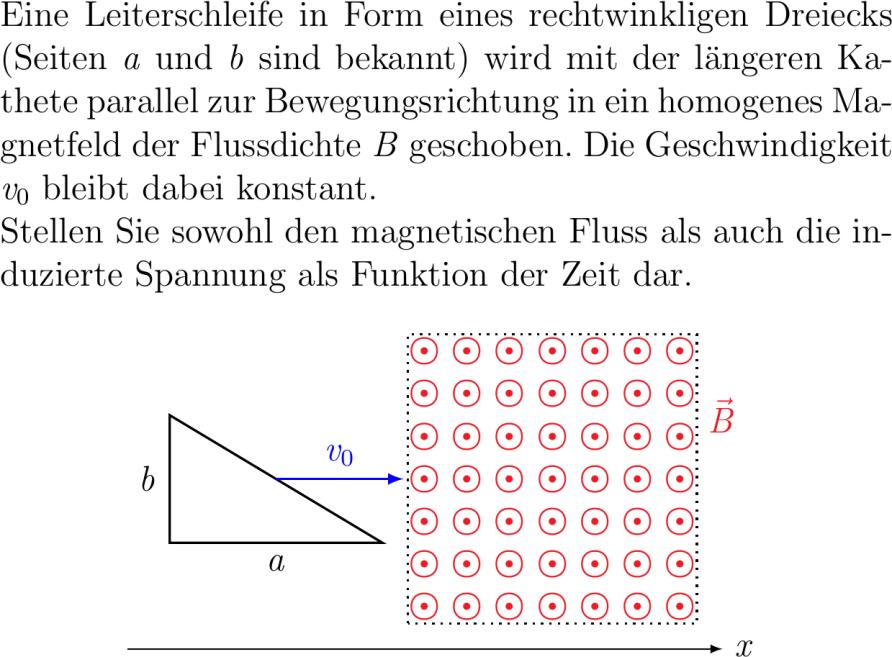
Eine Leiterschleife in Form eines rechtwinkligen Dreiecks Seiten a und b sind bekannt wird mit der längeren Kathete parallel zur Bewegungsrichtung in ein homogenes Magnetfeld der Flussdichte B geschoben. Die Geschwindigkeit v_ bleibt dabei konstant. Stellen Sie sowohl den magnetischen Fluss als auch die induzierte Spannung als Funktion der Zeit dar. figureH centering tikzpicturelatex %draw step.colorgray! - grid ; %fill circle .; draw - -.-.--.-. noderight x; draw thick --nodebelowa.--.--nodeleftb cycle; foreach x in .... foreach y in ...... node Red at xy bmodot; node Red at ..vecB; draw -thickblue ..--nodeabovev_ ..; draw dottedthick .. rectangle ..; tikzpicture figure
Solution:
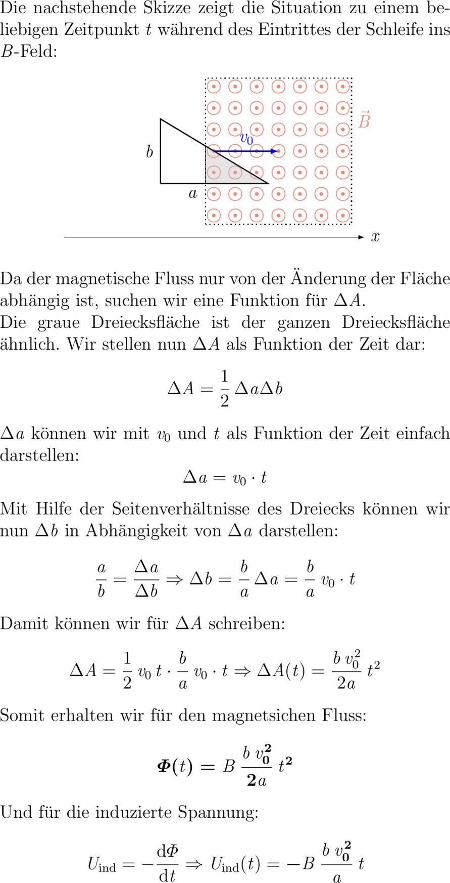
Die nachstehe Skizze zeigt die Situation zu einem beliebigen Zeitpunkt t währ des Erittes der Schleife ins B-Feld: figureH centering tikzpicturelatex %draw step.colorgray! - grid ; %fill circle .; draw - -.-.--.-. noderight x; foreach x in .... foreach y in ...... node Red! at xy bmodot; node Red! at ..vecB; draw dottedthick .. rectangle ..; scopexshift.cm draw thick --nodebelowxshift-.cma.--.--nodeleftb ; draw -thickblue ..--nodeabovev_ ..; draw fillgray fill opacity. .--..--.--cycle; scope tikzpicture figure Da der magnetische Fluss nur von der Änderung der Fläche abhängig ist suchen wir eine Funktion für Delta A. Die graue Dreiecksfläche ist der ganzen Dreiecksfläche ähnlich. Wir stellen nun Delta A als Funktion der Zeit dar: Delta AfracDelta aDelta b Delta a können wir mit v_ und t als Funktion der Zeit einfach darstellen: Delta av_ t Mit Hilfe der Seitenverhältnisse des Dreiecks können wir nun Delta b in Abhängigkeit von Delta a darstellen: fracabfracDelta aDelta bRa Delta bfracbaDelta afracbav_ t Damit können wir für Delta A schreiben: Delta Afracv_tfracbav_ t Ra Delta Atfracbv_^at^ Somit erhalten wir für den magnetsichen Fluss: boldsymbolvarPhitBfracbv_^at^ Und für die induzierte Spannung: U_mathrmind-fracmathrmdvarPhimathrmdtRa U_mathrmindtboldsymbol-Bfracbv_^at
Eine Leiterschleife in Form eines rechtwinkligen Dreiecks Seiten a und b sind bekannt wird mit der längeren Kathete parallel zur Bewegungsrichtung in ein homogenes Magnetfeld der Flussdichte B geschoben. Die Geschwindigkeit v_ bleibt dabei konstant. Stellen Sie sowohl den magnetischen Fluss als auch die induzierte Spannung als Funktion der Zeit dar. figureH centering tikzpicturelatex %draw step.colorgray! - grid ; %fill circle .; draw - -.-.--.-. noderight x; draw thick --nodebelowa.--.--nodeleftb cycle; foreach x in .... foreach y in ...... node Red at xy bmodot; node Red at ..vecB; draw -thickblue ..--nodeabovev_ ..; draw dottedthick .. rectangle ..; tikzpicture figure
Solution:
Die nachstehe Skizze zeigt die Situation zu einem beliebigen Zeitpunkt t währ des Erittes der Schleife ins B-Feld: figureH centering tikzpicturelatex %draw step.colorgray! - grid ; %fill circle .; draw - -.-.--.-. noderight x; foreach x in .... foreach y in ...... node Red! at xy bmodot; node Red! at ..vecB; draw dottedthick .. rectangle ..; scopexshift.cm draw thick --nodebelowxshift-.cma.--.--nodeleftb ; draw -thickblue ..--nodeabovev_ ..; draw fillgray fill opacity. .--..--.--cycle; scope tikzpicture figure Da der magnetische Fluss nur von der Änderung der Fläche abhängig ist suchen wir eine Funktion für Delta A. Die graue Dreiecksfläche ist der ganzen Dreiecksfläche ähnlich. Wir stellen nun Delta A als Funktion der Zeit dar: Delta AfracDelta aDelta b Delta a können wir mit v_ und t als Funktion der Zeit einfach darstellen: Delta av_ t Mit Hilfe der Seitenverhältnisse des Dreiecks können wir nun Delta b in Abhängigkeit von Delta a darstellen: fracabfracDelta aDelta bRa Delta bfracbaDelta afracbav_ t Damit können wir für Delta A schreiben: Delta Afracv_tfracbav_ t Ra Delta Atfracbv_^at^ Somit erhalten wir für den magnetsichen Fluss: boldsymbolvarPhitBfracbv_^at^ Und für die induzierte Spannung: U_mathrmind-fracmathrmdvarPhimathrmdtRa U_mathrmindtboldsymbol-Bfracbv_^at